Cobwebbing, linear approximation and stability
This applet shows a linear approximation to a non-linear difference equation close to an equilibrium, using cobwebbing. It can be used to investigate the accuracy of a linear approximation, or to motivate the linear stability criterion for equilibria of a first-order difference equation.
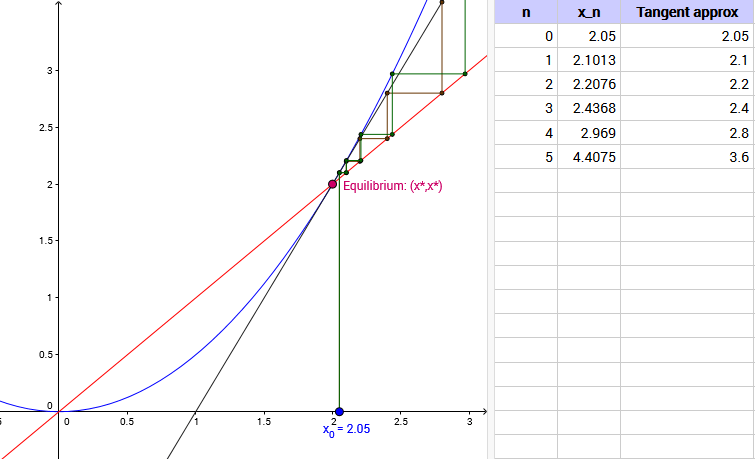
The plot shows a cobweb diagram for a difference equation $x_{n+1} = g(x_n)$. Move $x_0$ and click ‘Iterate’ to perform cobwebbing with the difference equation.
Click ‘Show equilibrium’ to highlight the equilibrium point on the diagram. Drag the pink point to select a different equilibrium.
Click ‘Show tangent’ to add a tangent line to the curve g(x) at the equilibrium point. What is the equation of the tangent line? What difference equation does it represent?
Click ‘Show tangent cobwebs’ to add in cobwebs for the tangent line. How do they compare to the cobwebs for the original difference equation? What happens as you move further away from x*? Closer to x*?
The spreadsheet to the right shows the values obtained by iterating the original difference equation, or its tangent approximation. How do the values compare?
When is the equilibrium x* stable? When is is unstable?
Hold shift and click & drag to move the view, hold shift and scroll the mouse wheel to zoom.
Other resources: