Visualising row, column and solution spaces
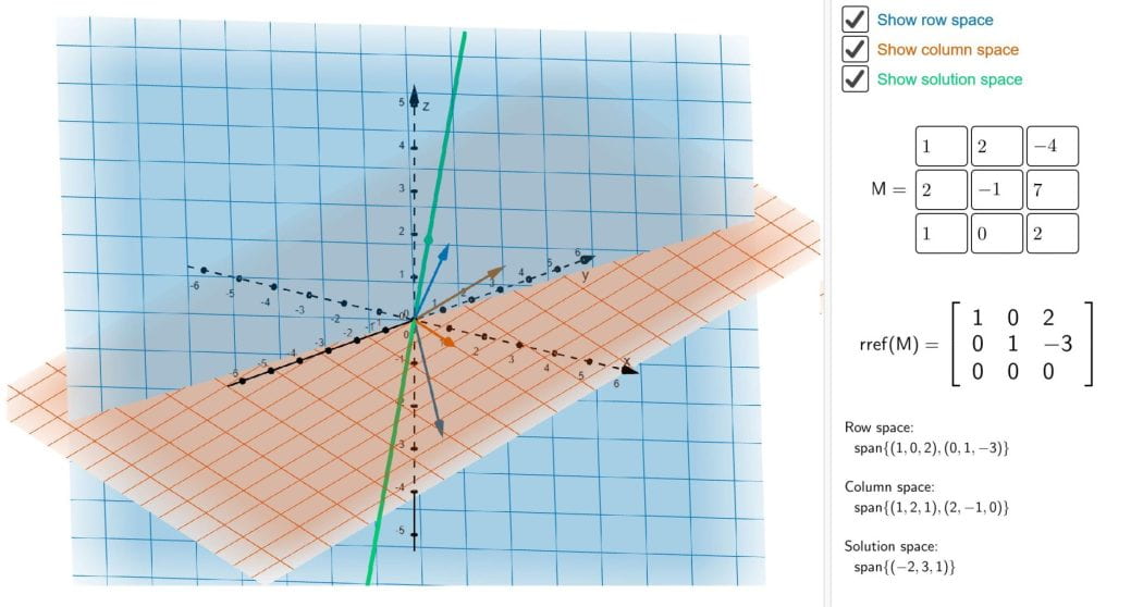
This applet shows the row, column, and solution spaces of a 3×3 matrix M. The row space is shown in blue, the column space is shown in orange, and the solution space is shown in green.
You can edit the matrix to view how these spaces change, and you can toggle the visibility of the three spaces by clicking the checkboxes on the right.
Some things you may notice are:
- The row and column spaces always have the same dimension, equal to the rank of M
- The dimension of the row/column spaces and the dimension of the solution space always sums to 3, in accordance with the rank-nullity theorem
- The row space is always orthogonal to the solution space of M
Here are some interesting matrices to try:
\[ \begin{bmatrix} 1 & 2 & -1 \\ 2 & 4 & -2 \\ 1 & 2 & -1 \end{bmatrix} \]
Before you put this in the applet, look at the columns of this matrix – what do you notice? Can you guess what the column space will look like?
\[ \begin{bmatrix} 1 & 2 & -4 \\ 2 & -1 & 7 \\ 1 & 0 & 3 \end{bmatrix} \]
What is the solution space in this case? (Hint: remember that the span of an empty set is the ‘trivial’ subspace consisting of just the 0 vector.)
The 0 matrix:
\[ \begin{bmatrix} 0 & 0 & 0\\ 0 & 0 & 0 \\ 0 & 0 & 0 \end{bmatrix} \]
What is the row and column space in this case?
Other resources: